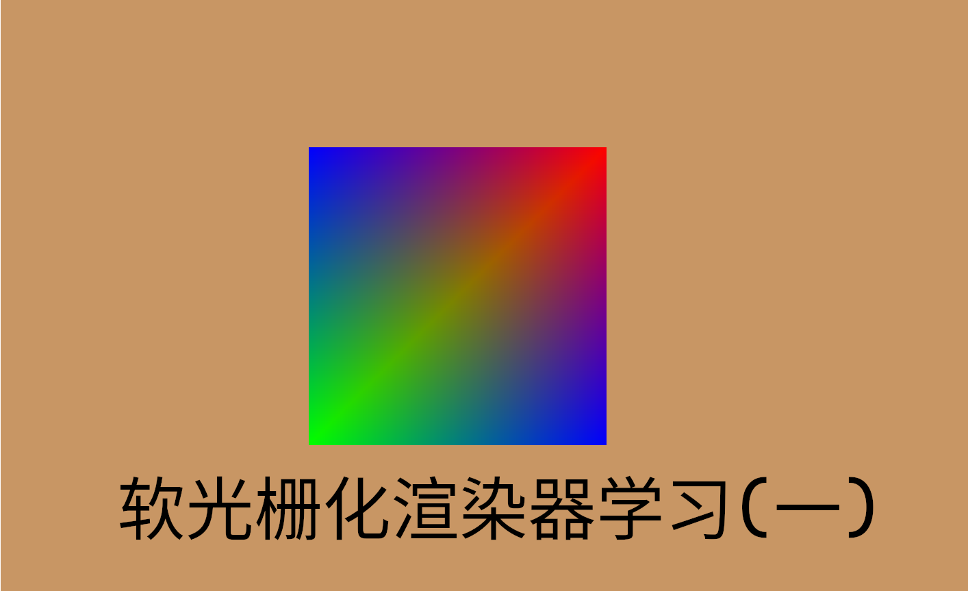
软光栅化渲染器学习(二)

软光栅化渲染器学习(一)

深度测试

深度测试通过标准化的z值，判断图元的前后关系，从而判断可见性。

在Renderer中新增一个深度缓冲：

Renderer::Renderer(Window &window)
{
    // ...
    depth_buffer = new float[window.width * window.height];
    depth_buffer_size = window.width * window.height;
}

void Renderer::ClearDepth()
{
    for (size_t i = 0; i < depth_buffer_size; i++)
        depth_buffer[i] = 1.0f;
}

每次清除深度缓冲时，将值赋为1，因为我们规定深度缓冲中的z值为$[0,1]$的，且0表示最近，1表示最远。

在软渲染器中，我们可以在光栅化调用片段着色器之前，进行深度测试。然而，通常这在GPU渲染管线中是提前深度测试(Early Z)，因为片段着色器可以改变顶点深度，理论上只能在之后进行深度测试。但在确保深度不改变，以及未开启透明度测试等的情况下，GPU会将深度测试提前来提高性能。

float z_ndc = alpha * vertices[0].position.z + beta * vertices[1].position.z + gamma * vertices[2].position.z;
float zbuffer_val = z_ndc * 0.5f + 0.5f;
if (depth_buffer[i + j * window->width] < zbuffer_val) continue; // 深度缓冲的像素比要绘制的像素还近，说明不用绘制了
else depth_buffer[i + j * window->width] = zbuffer_val;

绘制模型

Assimp加载模型

我们使用 Open Asset Importer Library（简称Assimp）这个模型导入库来加载3D模型，本文所用的模型来自github开源项目Tiny Renderer。

定义以下的Vertex和Mesh类用于存放加载的数据：

struct Vertex
{
    vec4f position;
    vec4f color;
    vec2f texCoords;
    vec3f normal;
};

struct Mesh
{
    std::vector<Vertex> vertices;
    std::vector<uint32_t> indices;
    Mesh(std::vector<Vertex> vertices, std::vector<uint32_t> indices)
        : vertices(vertices), indices(indices) {}
};

接着运用assimp的API，实现加载指定模型文件：

class Model
{
  public:
    Model(const std::string &filePath)
    {
        Assimp::Importer importer;
        const aiScene *scene = importer.ReadFile(filePath, aiProcess_Triangulate);
        if (!scene || scene->mFlags & AI_SCENE_FLAGS_INCOMPLETE || !scene->mRootNode)
        {
            std::cout << "ERROR::ASSIMP::" << importer.GetErrorString() << std::endl;
            return;
        }
        ProcessNode(scene->mRootNode, scene);
    }
  private:
    void ProcessNode(aiNode *node, const aiScene *scene)
    {
        // 处理节点所有的网格（如果有的话）
        for (unsigned int i = 0; i < node->mNumMeshes; i++)
        {
            aiMesh *mesh = scene->mMeshes[node->mMeshes[i]];
            meshes.push_back(ProcessMesh(mesh, scene));
        }
        // 接下来对它的子节点重复这一过程
        for (unsigned int i = 0; i < node->mNumChildren; i++)
        {
            ProcessNode(node->mChildren[i], scene);
        }
    }
    Mesh ProcessMesh(aiMesh *mesh, const aiScene *scene)
    {
        std::vector<Vertex> vertices;
        std::vector<uint32_t> indices;
        for (unsigned int i = 0; i < mesh->mNumVertices; i++)
        {
            Vertex vertex;
            vertex.position = vec4f(mesh->mVertices[i].x, mesh->mVertices[i].y, mesh->mVertices[i].z, 1.0f);
            if (mesh->HasNormals())
            {
                vertex.normal = vec3f(mesh->mNormals[i].x, mesh->mNormals[i].y, mesh->mNormals[i].z);
            }
            // 由于我们要处理的文件是.obj类型，.obj文件只能存储一套纹理坐标，因此存0号的纹理坐标即可。
            if (mesh->HasTextureCoords(0))
            {
                vertex.texCoords = vec2f(mesh->mTextureCoords[0][i].x, mesh->mTextureCoords[0][i].y);
            }
            vertices.push_back(vertex);
        }
        for (unsigned int i = 0; i < mesh->mNumFaces; i++)
        {
            aiFace face = mesh->mFaces[i];
            for (unsigned int j = 0; j < face.mNumIndices; j++)
                indices.push_back(face.mIndices[j]);
        }
        return Mesh(vertices, indices);
    }
  public:
    std::vector<Mesh> meshes;
};

绘制模型时，遍历mesm的indices数组，得到每个三角形面片对应的顶点，再调用绘制三角形的方法即可：

void Renderer::DrawMesh(const Mesh &mesh, RenderMode mode)
{
    for (size_t i = 0; i < mesh.indices.size(); i += 3)
    {
        uint32_t a = mesh.indices[i];
        uint32_t b = mesh.indices[i + 1];
        uint32_t c = mesh.indices[i + 2];
        DrawTriangle({mesh.vertices[a], mesh.vertices[b], mesh.vertices[c]}, mode);
    }
}

线框模式下，绘制的"african_head.obj"模型如下：

纹理加载

选择一张对应模型的纹理贴图，用stb_image库进行加载。定义如下Texture类：

class Texture
{
  public:
    Texture(const std::string &filePath, bool flipUV = false)
    {
        stbi_set_flip_vertically_on_load(filpUV);
        data = stbi_load(filePath.c_str(), &width, &height, &channels, 0); // 强制RGBA
        if (!data)
        {
            std::cout << "Cannot Load Texture!" << std::endl;
            return;
        }
    }
    enum SampleMode
    {
        Nearest,
        Billinear
    };
    int height;
    int width;
    int channels;
    unsigned char *data;
    vec4f Sample(float u, float v, SampleMode mode)
    {
        if (mode == Nearest)
        {
            // 处理纹理坐标超出[0,1]范围的情况
            u = std::fmod(u, 1.0f);
            v = std::fmod(v, 1.0f);
            if (u < 0) u += 1.0f;
            if (v < 0) v += 1.0f;

            // 转换为像素坐标
            int x = static_cast<int>(u * (width - 1));
            int y = static_cast<int>(v * (height - 1));
            int idx = (y * width + x) * channels;
            uint8_t r = data[idx];
            uint8_t g = data[idx + 1];
            uint8_t b = data[idx + 2];
            return vec4f(r / 255.0f, g / 255.0f, b / 255.0f, 1);
        }
        else if (mode == Billinear)
        {
            u = u * width - 0.5f;
            v = v * height - 0.5f;

            int x0 = static_cast<int>(std::floor(u)) % width;
            int y0 = static_cast<int>(std::floor(v)) % height;
            int x1 = x0 + 1, y1 = y0 + 1;

            // 处理边界
            x0 = std::max(0, std::min(x0, width - 1));
            y0 = std::max(0, std::min(y0, height - 1));
            x1 = std::max(0, std::min(x1, width - 1));
            y1 = std::max(0, std::min(y1, height - 1));

            // 获取四个邻近像素
            auto fetch = [&](int x, int y) {
                int offset = (y * width + x) * channels;
                return vec4f(
                    data[offset] / 255.0f,
                    data[offset + 1] / 255.0f,
                    data[offset + 2] / 255.0f,
                    1.0f);
            };

            vec4f p00 = fetch(x0, y0);
            vec4f p01 = fetch(x0, y1);
            vec4f p10 = fetch(x1, y0);
            vec4f p11 = fetch(x1, y1);

            // 插值权重
            float fracX = u - x0;
            float fracY = v - y0;

            // 双线性插值
            vec4f lerpBottom = p00 * (1 - fracX) + p10 * fracX;
            vec4f lerpTop = p01 * (1 - fracX) + p11 * fracX;
            return lerpBottom * (1 - fracY) + lerpTop * fracY;
        }
        return vec4f();
    }
};

这里提供了两种采样方式，分别是邻近像素采样以及双线性插值采样。

stb_image加载图片时，默认情况下像素是从左上角开始排列存储的，如果指定flipUV，则是从图片的左下角开始排列存储。存储顺序会影响到采样的纹理坐标，从上面的代码中可见，我们是通过int idx = (y * width + x) * channels;来判断要采哪个像素的，也就是认为图片存储是从左上角开始的，因而我们的纹理坐标系统也应该以左上角为原点。不同的图形API有不同的标准，如DirectX中纹理坐标以左上角为原点，而OpenGL中纹理坐标以左下角为原点。

标准不统一，导致很容易出现纹理上下颠倒的情况。在加载模型的对应纹理时，如果纹理上下颠倒，有两种途径解决：一是在加载纹理时指定上下翻转；二是在加载模型时，指定顶点uv坐标上下翻转（可以在Assimp加载模型时指定）。这里我们采用第一种解决方法。

纹理附着

这里选用"african_head_diffuse.tga"这张纹理（在原项目中是用来确定Blinn-Phong模型的diffuse项的），在加载时指定该纹理需要上下翻转。

在绘制三角形时，对纹理坐标按照其他属性一样进行透视矫正插值。同时仿照图形API，我们将片段着色器的代码单独提取出来。

for (int i = (int)minx; i <= (int)maxx; i++)
    for (int j = (int)miny; j <= (int)maxy; j++)
    {
        vec2f p(i + 0.5f, j + 0.5f);
        vec2f s0 = triangle[0].position.xy() - p;
        vec2f s1 = triangle[1].position.xy() - p;
        vec2f s2 = triangle[2].position.xy() - p;
        float Sa = vector_cross(s1, s2);
        float Sb = vector_cross(s2, s0);
        float Sc = vector_cross(s0, s1);
        if (!((Sa >= 0 && Sb >= 0 && Sc >= 0) || (Sa <= 0 && Sb <= 0 && Sc <= 0))) continue;
        float S = Sa + Sb + Sc;
        float alpha = Sa / S, beta = Sb / S, gamma = Sc / S; // 重心坐标

        // 提前深度测试
        float z_ndc = alpha * triangle[0].position.z + beta * triangle[1].position.z + gamma * triangle[2].position.z;
        float zbuffer_val = z_ndc * 0.5f + 0.5f;
        if (depth_buffer[i + j * window->width] < zbuffer_val) continue; 
        else depth_buffer[i + j * window->width] = zbuffer_val;

        // 透视矫正插值
        float reverse_wt = alpha / triangle[0].position.w + beta / triangle[1].position.w + gamma / triangle[2].position.w;
        Vertex curPixel;
        
        curPixel.color = (alpha * triangle[0].color / triangle[0].position.w 
                    + beta * triangle[1].color / triangle[1].position.w
                    + gamma * triangle[2].color / triangle[2].position.w) / reverse_wt;

        curPixel.normal = (alpha * triangle[0].normal / triangle[0].position.w 
                    + beta * triangle[1].normal / triangle[1].position.w 
                    + gamma * triangle[2].normal / triangle[2].position.w) / reverse_wt;

        curPixel.texCoords = (alpha * triangle[0].texCoords / triangle[0].position.w 
                            + beta * triangle[1].texCoords / triangle[1].position.w 
                            + gamma * triangle[2].texCoords / triangle[2].position.w) / reverse_wt;

        // 片段着色器
        vec3f fragColor = vector_clamp(FragmentShader(curPixel));
        SetPixel(i, j, fragColor.r * 255, fragColor.g * 255, fragColor.b * 255);
    }

vec3f Renderer::FragmentShader(Vertex p)
{
    vec3f color = texture->Sample(p.texCoords.u, p.texCoords.v, Texture::SampleMode::Nearest).xyz();
    return color;
}

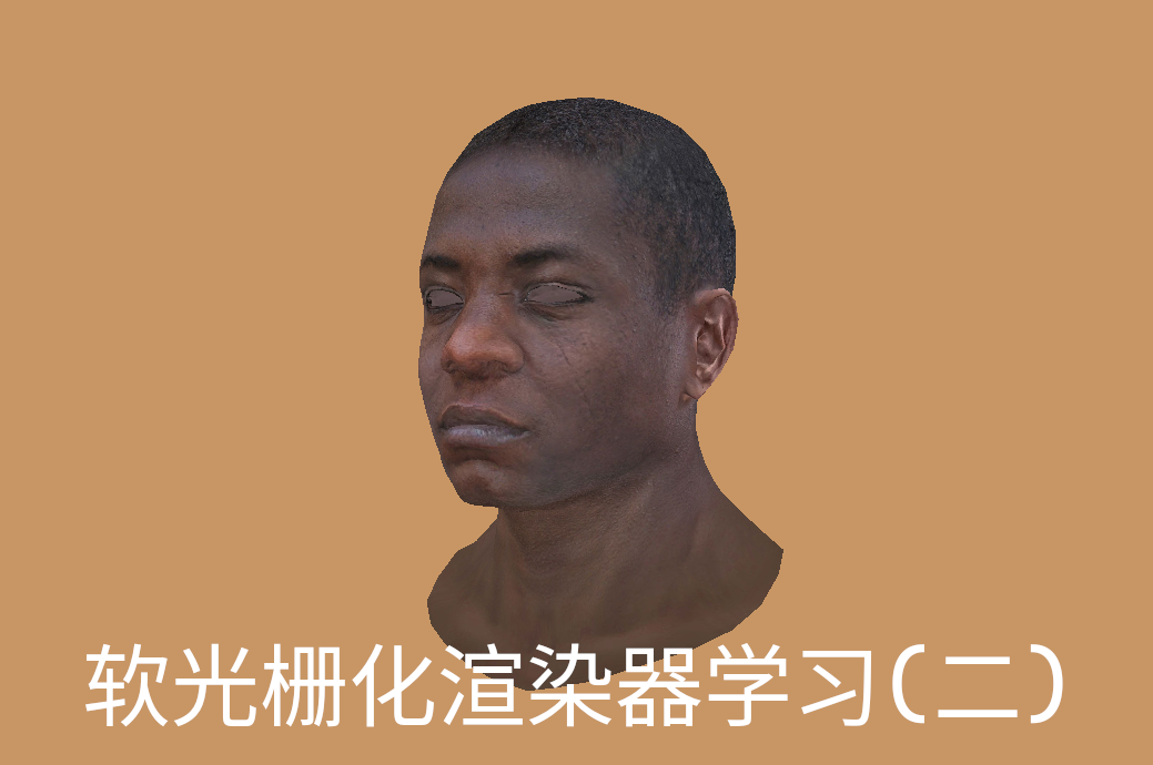
结果如下：

剔除与裁剪

剔除(Culling)是指判断某些几何体是否完全不需要绘制，并直接丢弃以提高效率，其不改变顶点；而裁剪(Clipping)则是对部分可见、部分不可见的几何体进行切割（涉及到修改顶点），使其只保留在视锥体内的可见部分。两者都是用于提高渲染效率和保证正确性的方法，但在图形管线中各司其职。

面剔除

面剔除(Face Culling)将背对相机的面片直接舍弃。对于大多数模型（封闭体）来说，背对相机的三角形一定不可见，因为它们总会被正对相机的面所遮挡。面剔除的原理很简单，即约定好三角形顶点的环绕方向，对于顶点逆时针环绕的三角形，其朝向相机正面(z轴正方向)，这也符合右手定则，对于逆时针环绕的三个顶点$A,B,C$，有：

$$\overrightarrow{AB}\times\overrightarrow{BC}>0$$

面剔除通常在顶点变换之后，光栅化之前，具体代码如下：

void Renderer::DrawTriangle(std::vector<Vertex> vertices, RenderMode mode)
{
    // ...
    vec2f ab = vertices[1].position.xy() - vertices[0].position.xy();
    vec2f bc = vertices[2].position.xy() - vertices[1].position.xy();
    if (vector_cross(ab, bc) < 0)
        return; // 直接舍弃该三角形
    // ...
}

使用面剔除后，再用线框模式绘制上面的模型，可以看出模型背面的三角形被剔除了：

视锥剔除

视锥剔除需要在CPU完成，GPU渲染管线是不会自动做的。其位于观察变换之后，在观察空间中将完全不在视锥内的图元舍弃。

判断一个点是否在视锥外，可以判断其与视锥六个面的位置关系。
对于$near$和$far$平面，可以简单地用顶点的z值判断。对于另外四个平面，可以计算出对应向外的法向量与顶点坐标对应的向量点乘，来判断在该平面的内外。

例如，对于上方的平面，其平行于x轴，列出平面方程：

$$By+Cz=0$$

将近平面的顶端中点值代入，即点$(0,\frac{h}{2},-n)$，得：

$$B\cdot\frac{h}{2}-Cn=0$$

取$B=n,C=\frac{h}{2}$，得到平面法向量$(0,n,\frac{h}{2})$，且该法向量向外。

类似地，可以得到右侧平面法向量为$(n,0,\frac{w}{2})$，其余同理。

因此视锥剔除的代码如下：

bool Frustum::Contain(vec3f p) const
{
    float radians_fov = fov * std::numbers::pi / 180.0f;
    float half_h = near * tan(0.5f * radians_fov);
    float half_w = half_h * aspect;
    return vector_dot(vec3f(near, 0.0, half_w), p) <= 0.0f 
        && vector_dot(vec3f(-near, 0.0, half_w), p) <= 0.0f 
        && vector_dot(vec3f(0.0f, near, half_h), p) <= 0.0f 
        && vector_dot(vec3f(0.0f, -near, half_h), p) <= 0.0f 
        && -p.z >= near 
        && -p.z <= far;
}

void Renderer::DrawTriangle(std::vector<Vertex> vertices, RenderMode mode)
{
    // ...
    bool should_cull = true;
    for (auto &vertex : vertices)
    {
        if (camera.GetFrustum().Contain(vertex.position.xyz()))
        {
            should_cull = false;
            break;
        }
    }
    if (should_cull) return;
    // ...
}

实际应用中，我们往往检测的是物体的包围盒来判断是否要剔除，这样效率更高。

裁剪

裁剪与视锥剔除都是将图元限制在视锥可视范围内，但是裁剪是指投影变换之后，透视除法之前，在齐次裁剪空间进行的过程。在GPU渲染管线中，这一步是GPU自动完成的，也是为确保正确性而必须的。可以认为，在这之前的CPU的视锥剔除是粗粒度的，而裁剪则是细粒度的。裁剪包含了视锥剔除的功能，也就是将完全不再视锥内的图元舍弃，但是毕竟这些图元越早舍弃越好，因此才会有CPU的视锥剔除。

经过投影变换之后，判断一个点$(x,y,z,w)$在视锥内的方法极为简单，就是判断$x\in [-w,w],y\in[-w,w],z\in[-w,w]$。

但裁剪要将位于边界上的，部分可见部分不可见的三角形，分割并保留可见的部分，这涉及到三维空间的多边形裁剪算法。

Sutherland–Hodgman多边形裁剪算法

该算法支持给定一组平面作为裁剪空间，对凸多边形进行裁剪。这里，我们只考虑对三角形的裁剪，对每个顶点，其裁剪空间就是三个坐标的$[-w,w]$，共六个平面。

算法的核心思想是，对于给定的一组顶点，依次用平面进行裁剪，对于一个特定平面，判断按顺序相邻的两顶点（称为前顶点与后顶点）与平面的位置关系，按规则保留原顶点并新增交点。规则如下：

顶点与平面关系	操作
内 -> 内	只保留后顶点
外 -> 外	全部丢弃
内 -> 外	只保留交点
外 -> 内	保留后顶点和交点

对于交点的计算，有一种十分巧妙的方法来简化计算：定义函数$f(\mathbf{p})$表示顶点到对应平面的带符号距离，其中$f(\mathbf{p})>0$表示点在平面内，$f(\mathbf{p})<0$表示点在平面外。

对于要插值的交点$\mathbf{v}_t=\mathbf{v}_0+t(\mathbf{v}_1 - \mathbf{v}_0),t\in [0,1]$，它到平面的距离必为0，因此满足：

$$f(\mathbf{v}_t)=f(\mathbf{v}_0)+t(f(\mathbf{v}_1)-f(\mathbf{v}_0))=0$$

故

$$t=\frac{f(\mathbf{v}_0)}{f(\mathbf{v}_0)-f(\mathbf{v}_1)}$$

得到插值系数之后，对顶点的位置和其他所有顶点属性进行线性插值，因为齐次裁剪空间内位置是线性变化的，只需线性插值即可。

bool InsidePlane(const Vertex &v, int plane)
{
    const auto &p = v.position;
    switch (plane)
    {
    case 0: return p.x >= -p.w; // Left
    case 1: return p.x <= p.w;  // Right
    case 2: return p.y >= -p.w; // Bottom
    case 3: return p.y <= p.w;  // Top
    case 4: return p.z >= -p.w; // Near
    case 5: return p.z <= p.w;  // Far
    }
    return false;
}

Vertex ComputeIntersection(const Vertex &v0, const Vertex &v1, int plane)
{
    auto f = [&](const vec4f &p) {
        switch (plane)
        {
        case 0: return p.x + p.w; // Left
        case 1: return p.x - p.w; // Right
        case 2: return p.y + p.w; // Bottom
        case 3: return p.y - p.w; // Top
        case 4: return p.z + p.w; // Near
        case 5: return p.z - p.w; // Far
        }
        return 0.0f;
    };

    float t = f(v0.position) / (f(v0.position) - f(v1.position));
    Vertex out;

    // 线性插值
    out.position = vector_lerp(v0.position, v1.position, t);
    out.color = vector_lerp(v0.color, v1.color, t);
    out.texCoords = vector_lerp(v0.texCoords, v1.texCoords, t);
    out.normal = vector_normalize(vector_lerp(v0.normal, v1.normal, t));

    return out;
}

std::vector<Vertex> ClipTriangle(const std::vector<Vertex> &triangle)
{
    std::vector<Vertex> poly(triangle.begin(), triangle.end());

    // 依次对 6 个裁剪平面执行 Sutherland–Hodgman
    for (int plane = 0; plane < 6; ++plane)
    {
        std::vector<Vertex> newPoly;

        for (size_t i = 0; i < poly.size(); ++i)
        {
            const Vertex &current = poly[i];
            const Vertex &next = poly[(i + 1) % poly.size()];

            bool currInside = InsidePlane(current, plane);
            bool nextInside = InsidePlane(next, plane);

            if (currInside && nextInside)
            {
                // 内 -> 内：只保留后顶点
                newPoly.push_back(next);
            }
            else if (currInside && !nextInside)
            {
                // 内 -> 外：保留交点
                Vertex inter = ComputeIntersection(current, next, plane);
                newPoly.push_back(inter);
            }
            else if (!currInside && nextInside)
            {
                // 外 -> 内：保留交点和后顶点
                Vertex inter = ComputeIntersection(current, next, plane);
                newPoly.push_back(inter);
                newPoly.push_back(next);
            }
            // 外 -> 外：全部丢弃
        }

        poly = std::move(newPoly);

        if (poly.empty())
        {
            return {}; // 完全在外部，直接丢弃
        }
    }
    return poly;
}

Sutherland–Hodgman算法完成后得到的一组顶点，有可能是多边形，因此还需要一步三角化(Triangulate)。一种简单的做法是扇形三角化，将一个顶点共用，其余顶点顺次连线段与共用顶点构成三角形。

std::vector<std::vector<Vertex>> Triangulate(const std::vector<Vertex> &poly)
{
    std::vector<std::vector<Vertex>> result;
    if (poly.size() < 3) return result;

    const Vertex &base = poly[0];
    for (size_t i = 1; i + 1 < poly.size(); ++i)
    {
        result.push_back({base, poly[i], poly[i + 1]});
    }
    return result;
}

std::vector<std::vector<Vertex>> ClipAndTriangulate(const std::vector<Vertex> &triangle)
{
    std::vector<Vertex> clipped = ClipTriangle(triangle);

    // 裁剪后没有有效顶点，则舍弃，相当于视锥剔除
    if (clipped.size() < 3)
        return {};

    return Triangulate(clipped);
}

---

参考资料：
https://github.com/VisualGMQ/rs-cpurenderer